Cartoonify an Image with OpenCV in Python
Introduction
Cartoonifying an image involves converting a regular photograph into a cartoon-style representation. It includes simplifying complex details, accentuating edges, reducing the number of colors, and applying artistic effects. This technique adds a whimsical and playful touch, turning ordinary images into visually appealing cartoons. It can be used for various purposes, such as creating avatars, designing comics, or adding a unique twist to digital artwork.
In This we are going to Cartoonify an Image using OpenCV
Open CV
OpenCV is a popular open-source computer vision library used for image processing tasks. It offers a comprehensive set of algorithms and functions that enable developers and researchers to perform various operations such as image manipulation, feature detection, and machine learning. With support for multiple programming languages, including C++, Python, and Java, OpenCV is widely accessible to a diverse range of users.
The library is organized into modules, providing modular functionality for core operations, image filtering, feature extraction, and more. This modular structure allows users to select and utilize the specific components needed for their projects. OpenCV has gained significant popularity due to its versatility and applicability in various fields. It finds applications in robotics, augmented reality, medical imaging, surveillance, and numerous other domains where computer vision is essential.
OpenCV’s success is attributed to its extensive community support, continuous development, and frequent updates. It remains actively maintained to ensure compatibility with modern hardware and software platforms. The library’s robustness, flexibility, and ease of use make it an invaluable resource for those working with computer vision and image processing tasks.
Step 1 — Installing OpenCV
To install OpenCV:
pip install opencv-python
Step 2 — Importing necessary libraries
Import the following libraries in your notebook –
- OpenCV
- easygui
- numpy
- matplotlib.pyplot
- imageio
import sys
import os
import cv2
import easygui
import numpy as np
import matplotlib.pyplot as plt
import imageio
Step 3 — Reading an image
Now for input, we need to select an image. Image can be selected from either your system or can be uploaded directly from the internet. Here, I’ve uploaded one from my system. For this, I’ve made use of easygui library.
ImagePath=easygui.fileopenbox()
img1=cv2.imread(ImagePath)
if img1 is None:
        print("Can not find any image. Choose appropriate file")
        sys.exit()
img1=cv2.cvtColor(img1,cv2.COLOR_BGR2RGB)
The image is stored in img. In case no file is selected or the uploaded file format is not selected then a message as “Can not find any image. Choose appropriate file” will be displayed.
The image is by default read in BGR color palette. We need to convert it in RGB format.
img1g=cv2.cvtColor(img1,cv2.COLOR_RGB2GRAY)
Step 4 — Median Blurring
3 types of blurring are available namely,
- Gaussian Blur
- Median Blur
- Bilateral Blur
Here, we perform median blurring on the image. The central element of the image is replaced by the median of all the pixels in the kernel area. This operation processes the edges while removing the noise.
img1b=cv2.medianBlur(img1g,3)
plt.imshow(img1b,cmap='gray')
plt.axis("off")
plt.title("AFTER MEDIAN BLURRING")
plt.show()
Step 5 — Edge Mask
The next step is to create the edge mask of the image. To do so, we make use of the adaptive threshold function.
Adaptive thresholding is the method where the threshold value is calculated for smaller regions and therefore, there will be different threshold values for different regions.
edges=cv2.adaptiveThreshold(img1b,255,cv2.ADAPTIVE_THRESH_MEAN_C,cv2.THRESH_BINARY,3,3)
plt.imshow(edges,cmap='gray')
plt.axis("off")
plt.title("Edge Mask")
plt.show()
Step 6 — Removing Noise
We need to get rid of the unwanted details of the image or the “noise”. In imaging, noise emerges as an artifact in the image that appears as a grainy structure covering the image.
To do so, we perform bilateral blurring.
img1bb=cv2.bilateralFilter(img1b, 15, 75, 75)
plt.imshow(img1bb,cmap='gray')
plt.axis("off")
plt.title("AFTER BILATERAL BLURRING")
plt.show()
Step 7 — Eroding and Dilating
Erosion —
- Erodes away the boundaries of the foreground object
- Used to diminish the features of an image.
Dilation —
- Increases the object area
- Used to accentuate features
kernel=np.ones((1,1),np.uint8)
img1e=cv2.erode(img1bb,kernel,iterations=3)
img1d=cv2.dilate(img1e,kernel,iterations=3)
plt.imshow(img1d,cmap='gray')
plt.axis("off")
plt.title("AFTER ERODING AND DILATING")
plt.show()
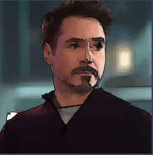
Step 8 — Stylization of an image
Now, we perform stylization on the image.
final=cv2.bitwise_and(final_img,final_img,mask=edges)
plt.imshow(final,cmap='gray')
plt.axis("off")
plt.title("FINAL")
plt.show()
The output is –